Reading Response for May 23

Reading Response for May 23

by Maria Glymour -
Number of replies: 6

This is a simulation exercise to illustrate how any specific sample and data analysis you conduct is just a single draw from a larger population and multiple possible iterations of the sample and analysis. 

Specify a hypothesis regarding a particular exposure and outcome and a binary effect modifier including specific measures of association (e.g., the relative risk or the odds ratio, specify the magnitudes of that association you anticipate: I suggest making everything cross-sectional for simplicity). Using the software of your choice, generate a population with 1000 people under a causal structure consistent with this hypothesis. Draw a simple random sample 100 individuals from this population and estimate the population average exposure-outcome association and the association stratified by your modifier of interest within this subset.  Repeat this 10 times and write the parameter estimates and CI each time.

Repeat the data set construction, setting the causal effect to the null.  Again repeat this 10 times and write the parameter estimate and CI each time (if you figure out how to automate it, run it 1000 times and post the histogram of the parameter estimates and p-values).

Please post your results from each of the 10 runs under the hypothesized effect and under the null and your code.

If you are flummoxed by this, note that example code is in Mayeda's simulation paper (which she posted last week) and in Glymour and Vittinghoff "Selection bias, just because it's possible doesn't mean it's plausible", published in Epidemiology in 2014.  But write the simulation in whatever language you prefer and don't worry too much about making beautiful code. 
In reply to Maria Glymour

Re: Reading Response for May 23

by Josh -

The research question I looked at was the association between smoking intensity and lung cancer.  I oversimplified the question by dichotomizing the exposure to be <25 pack years and >25 pack years.  My effect modifier was family history.  Not sure I did this correctly, but suggestions for future simulation are greatly appreciated.

Here are my results:

Effect Model (OR = 10)
Sample Main Effect OR OR (Fam_Hx = 1) OR (Fam_Hx = 0)
1 19.7 N Too Small 12.11
2 7.5 N Too Small 3.2
3 6.8 1.9 12.9
4 9 6 11.25
5 9.5 N Too Small 7
6 12.9 36 10.1
7 7.2 27 3.6
8 14.8 6.8 23
9 10.5 N Too Small 4.3
10 9.1 2.4 11.8


Null Model (OR = 1)
Sample Main Effect OR OR (Fam_Hx = 1) OR (Fam_Hx = 0)
1 0.9 0.7 1
2 1.4 1.2 1.6
3 2.1 1.6 2.3
4 0.9 0.7 1
5 1.3 2.1 1
6 1.6 5.3 1.1
7 1.1 1.1 1.2
8 0.6 2.8 0.3
9 0.8 1 0.7
10 0.9 0.4 1.4


I attached my code.

In reply to Josh

Re: Reading Response for May 23

by Natalie -

I hypothesized an interaction in the effect of BMI and alcohol use on breast density (continuous). I dichotomized BMI and alcohol use for simplicity in this example.

I was confused a bit as to the wording of the question -- I assumed that the null hypothesis was that there was no interaction between the two variables (NOT that there was no effect of the exposure on outcome), and that the alternative hypothesis was that there was an interaction (positive in my example). Therefore the PATE of the exposure on outcome under the alternative hypothesis in the first part would wrongly ignore this interaction, right? I presented the beta for the interaction parameter instead. 

Code is attached with histograms of the beta's and a list of the betas and SE's for 1/10 of the 1000 runs under each scenario.


In reply to Maria Glymour

Re: Reading Response for May 23

by Thomas Gaither -

I am studying the effect of hormone replacement therapy on diastolic blood pressure with age (>65 versus <65) as my effect modifier. Here is the results when my beta=2. 


Sample #1

HRT= 2.34 (2.07-2.61)

HRT (with modifier)= 2 (2-2)


Sample #2

HRT= 2.39 (2.12-2.66)

HRT (with modifier)= 2 (2-2)


Sample #3

HRT= 2.62 (2.37-2.97)

HRT (with modifier)= 2 (2-2)


Sample #4

2.33 (2.07-2.58)

HRT (with modifier)= 2 (2-2)


Sample #5

2.46 (2.18-2.74)

HRT (with modifier)= 2 (2-2)


Sample #6

2.75 (2.45-3.04)

HRT (with modifier)= 2 (2-2)


Sample #7

2.66 (2.40-2.92)

HRT (with modifier)= 2 (2-2)


Sample #8

2.36 (2.09-2.63)

HRT (with modifier)= 2 (2-2)


Sample #9

2.50 (2.23-2.77)

HRT (with modifier)= 2 (2-2)


Sample #10

2.41 (2.13-2.68)

HRT (with modifier)= 2 (2-2) 


Here are the null results:

Sample #1

-0.18 (-0.35- -0.003)

HRT (with modifier)= -0.03 (-0.19- 0.14)


Sample #2

-0.15 (-0.36- 0.05)

HRT (with modifier)= -0.03 (-0.21-0.14)


Sample #3

0.01 (-0.17-0.20)

HRT (with modifier)= 0.01 (-0.15-0.17)


Sample #4

0.0     (-0.19-0.19)

HRT (with modifier)= 0.16 (0.04-0.29)


Sample #5

0.16 (0.04-0.29)

HRT (with modifier)= -0.27 (-0.48- -0.07)


Sample #6

0.09 (-0.12- 0.30)

HRT (with modifier)= 0.24 (0.07-0.41)


Sample #7

0.01 (-0.18-0.20)

HRT (with modifier)= 0.03 (-0.11- 0.18)


Sample #8

0.07 (-0.11- 0.25)

HRT (with modifier)= 0.02 (-0.11- 0.15)


Sample #9

-0.03 (-0.23-0.17)

HRT (with modifier)= 0.25 (0.10-0.41)


Sample #10

-0.11 (-0.33-0.10)

HRT (with modifier)= 0.04 (-0.19-0.26) 


Overall: The simulation under the null often produces statistically significant results. In the first part of the simulation it looks like it over-estimates more than under-estimates the true effect. 

In reply to Maria Glymour

Re: Reading Response for May 23

by Bambeiha Asiimwe -

This is the question

#whether exclusively drinking spirits (spirit) versus exclusively drinking wine or beer (WOB) increases your risk of dying in the next 10 years
#the effect modifier is HIV infection because spirits are thought to act by causing inflammation
#inflammation could in turn be more dangerous to HIV-infected individuals compared to their HIV uninfected counterparts because inflammation is closely linked with HIV pathophysiology

Software=R

This is the causal structure

#10% of the population exclusively drink wob
#20% of the population exclusively drink spirit
#18% of the population is HIV-infected (as in South Africa)
#Population level 10 year risk of death=0.17
#HIV infection tripples your risk of death
#Spirit increases risk of death in those with HIV 1.5-fold 
#Spirit increases risk of death in those without HIV 1.2-fold
#assume that age is associated with risk of death but not with whether or not you drink spirit or wob

This is the structural code in R

spirit=rbinom(1000, 1, .2)
wob=rbinom(1000, 1, .1)
hiv=rbinom(1000, 1, .18)

library("rje")
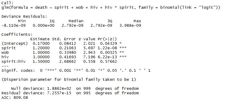
death=expit(0.17+1*wob+3*hiv+1.2*spirit+1.5*spirit*hiv)

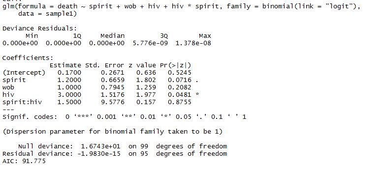
model1=glm(death~spirit+wob+hiv+hiv*spirit, family = binomial(link = "logit"))

summary(model1)

Now we sample

#but we can maybe make a dataframe first
alc=data.frame(age, spirit, wob, hiv, death)

#simple sampling

sample1<-alc[sample(1:nrow(alc), 100, replace=TRUE),]
model2=glm(death~spirit+wob+hiv+hiv*spirit, data=sample1, family = binomial(link = "logit"))
summary(model2)

Sample1model


Now we sample 10 times

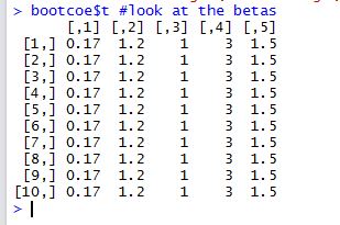
Somehow this is giving me the same coefficients all the time even after removing the seed.  I will return to it later.


library("boot")
#try something else
tensamples=function(data,indices){
data=alc #let boot to select sample
lm.out=glm(death ~ spirit + wob + hiv + hiv*spirit, data = alc, family = binomial(link = "logit"))
return(lm.out$coefficients)
}

NN=100
tensamples(alc,1:NN)

bootcoe=boot(alc,tensamples,R=10) #generate 10 random samples
bootcoe$t #look at the betas

coeffcients1


I will proceed to setting the causal structure to the null after figuring out why it is giving me the same coefficients all the time!


In reply to Bambeiha Asiimwe

Re: Reading Response for May 23

by Bambeiha Asiimwe -

I think i know why it is giving bad coefficients: wrong xpit function

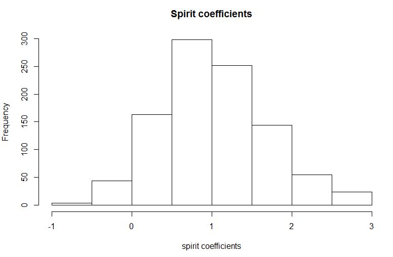
This is the histogram of the more correct coefficients (1000 runs) under the null hypothesis for spirit.  Its not even spirit coefficients, it should be "spirit odds ratios"

I am yet to figure out why it is giving some negative coefficients, and a few that are too outlying on the upper end.

In reply to Maria Glymour

Re: Reading Response for May 23

by Danielle -

I tried to post this yesterday but had both internet and myaccess troubles.  please find my attempt at this assignment attached including an excel spreadsheet with the two model's outputs, 2 STATA do files, and  2 STATA data files.  


My proposed model was looking at CF patients using WFL percentile at age 2 as a predictor of lung function at age 18.  The binary mediator was use of supplementation with formulas in the intervening time yes/no.


It has been a great class thank you all.


Danielle