
I am skipping this week.
I will also be skipping my response this week.
Specify a hypothesis regarding a particular exposure and outcome and a binary effect modifier including specific measures of association (specify the magnitudes of that association you anticipate: I suggest making everything cross-sectional). Using the software of your choice, generate a population with 1000 people under a causal structure consistent with this hypothesis. Draw a simple random sample 100 individuals from this population and estimate the population average exposure-outcome association and the association stratified by your modifier of interest within this subset. Repeat this 10 times and write the parameter estimates and CI each time.
Exposure (a): rainfall as measured as a deviation from long-term trends, a continuous measure capturing drought/extreme rainfall and normalized
Outcome (y): BMI among children under 5
Effect modifier (w): urban vs rural residence
Data generating rules:
n <- 1000
a <- rnorm(n, 0, 1)
w <- rbinom(n, 1, 0.3)
y_e <- runif(n)
y <- 0.1*a - 0.2*w - 0.1*a*w + y_e
Expected effect sizes:
Among urban (w = 1) = 0
Among rural (w = 0) = 0.1
Prevalence of urban = 0.3
Among total population: 0*0.3 + 0.1*(1-0.3) = 0.07
Results for each sample of 100 individuals
|
Sample number |
Effect of rainfall deviation (95% CI) |
Effect of rainfall deviation among urban (95% CI) |
Effect of rainfall deviation among rural (95% CI) |
|
1 |
0.021 (-0.035, 0.077) |
-0.055 (-0.15, 0.043) |
0.058 (-0.011, 0.13) |
|
2 |
0.085* (0.014, 0.16) |
-0.065 (-0.27, 0.14) |
0.11** (0.032, 0.18) |
|
3 |
0.0035 (-0.059, 0.066) |
-0.079 (-0.20, 0.40) |
0.043 (-0.020, 0.12) |
|
4 |
0.077** (0.023, 0.13) |
0.052 (-0.059, 0.15) |
0.086* (0.021, 0.15) |
|
5 |
0.089** (0.038, 0.14) |
0.037 (-0.048, 0.12) |
0.12*** (0.056, 0.19) |
|
6 |
0.078* (0.018, 0.14) |
-0.12 (-0.069, 0.27) |
0.11*** (0.052, 0.18) |
|
7 |
0.13*** (0.072, 0.19) |
0.10 (-0.055, 0.15) |
0.14*** (0.070, 0.20) |
|
8 |
0.072* (0.014, 0.13) |
0.050 (-0.035, 0.18) |
0.086* (0.010, 0.16) |
|
9 |
0.15*** (0.086, 0.21) |
0.073 (0.052) |
0.17*** (0.099, 0.25) |
|
10 |
0.066 (-0.0016, 0.013) |
0.022 (-0.090, 0.13) |
0.095* (0.0072, 0.18) |
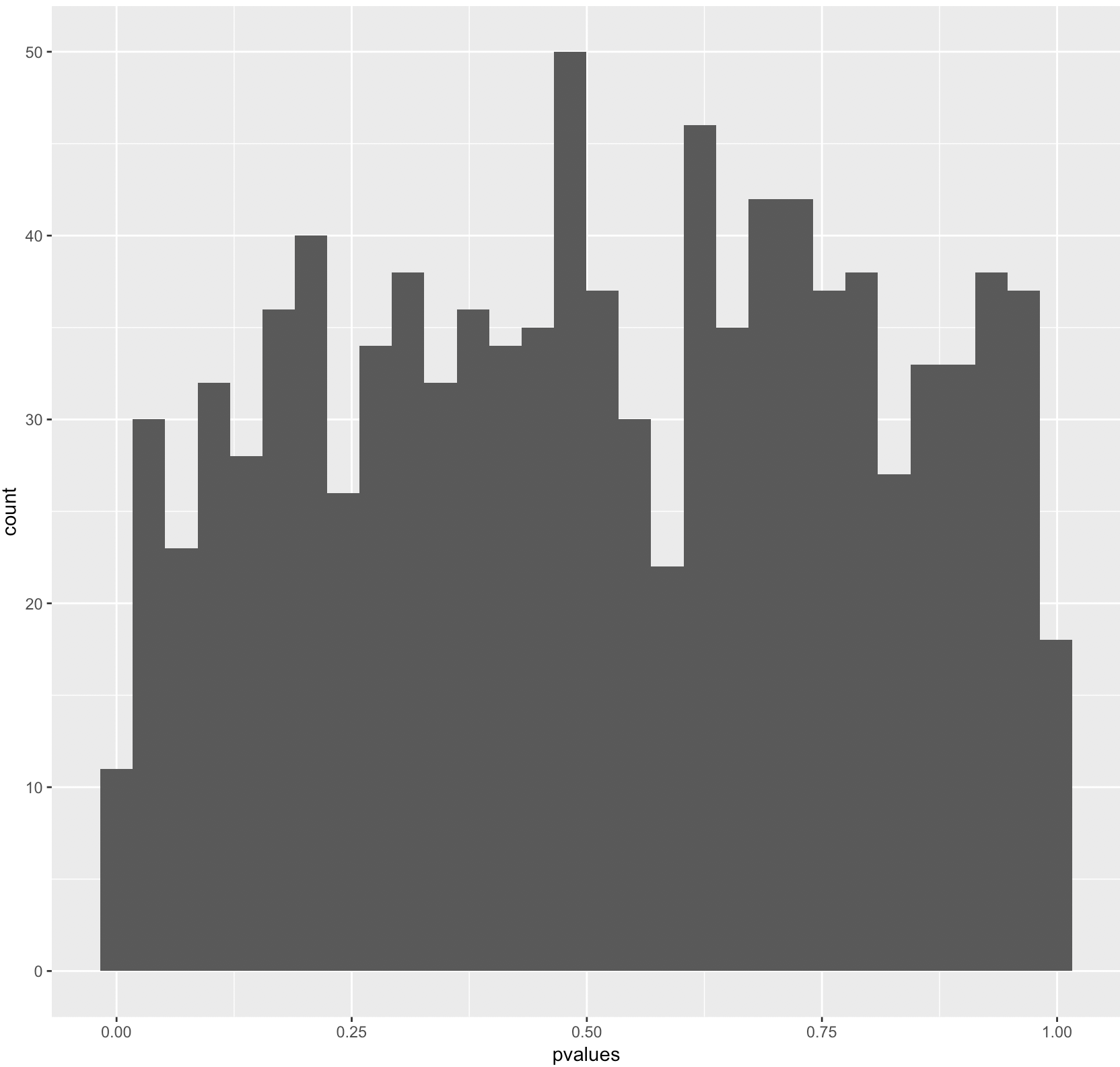
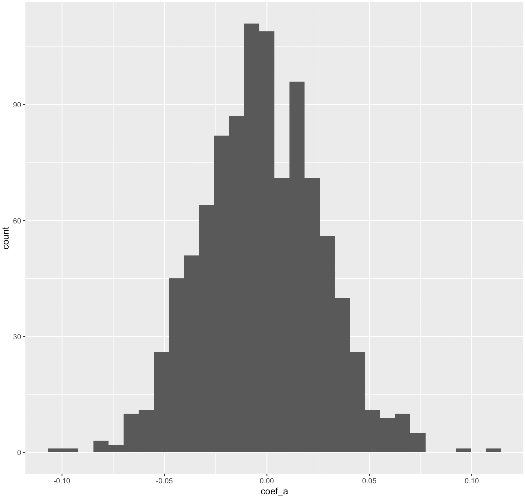
Repeat the data set construction, setting the causal effect to the null. Again repeat this 10 times and write the parameter estimate and CI each time (if you figure out how to automate it, run it 1000 times and post the histogram of the parameter estimates and p-values).
See attached histograms
Use your code above and also a canned software command to estimate statistical power to detect the difference in means under the settings below:
Note: see attachment for R code and simulation
*n=100, μ0=.02, μ1=.12, SD=1, α=.05
Power = 0.07
*n=100,μ0=.02, μ1=.12, SD=2, α=.05
Power = 0.04
*n=500, μ0=.3, μ1=.3, SD=1, α=.05
Power = 0.025
HA: Physical activity is associated with decreased systolic blood pressure and this effect is greater in wealthier people (>100FPL vs not).
gen physact = rpoisson(20)
gen poor = runiform()<.40
gen sbp_e = rnormal(0,1)
gen sbp = 120 -0.90*physact + 1.1*poor + 0.20*physact*poor + sbp_e
|
Pop avg effect of physact |
Avg effect of physact among high income (poor=0) |
Avg effect of physact among low income (poor=1) |
|
-0.91 (-1.01, -0.81) |
-0.92 (-0.96, -0.87) |
-0.73 (-0.80, -0.67) |
|
-0.87 (-0.99, -0.75) |
-0.89 (-0.96, -0.83) |
-0.76 (-0.84, -0.68) |
|
-0.91 (-1.03, -0.80) |
-0.92 (-0.98, -0.87) |
-0.67 (-0.75, -0.60) |
|
-0.82 (-0.93, -0.71) |
-0.94 (-0.99, -0.89) |
-0.71 (-0.77, -0.66) |
|
-0.91 (-1.03, -0.80) |
-0.94 (-1.00, -0.88) |
-0.68 (-0.76, -0.59) |
|
-0.80 (-0.91, -0.69) |
-0.90 (-0.94, -0.86) |
-0.61 (-0.68, -0.53) |
|
-0.87 (-0.99, -0.75) |
-0.92 (-0.98, -0.87) |
-0.66 (-0.75, -0.58) |
|
-0.90 (-1.03, -0.77) |
-0.95 (-1.00, -0.89) |
-0.69 (-0.79, -0.59) |
|
-0.85 (-0.97, -0.72) |
-0.95 (-1.00, -0.90) |
-0.74 (-0.82, -0.65) |
|
-0.83 (-0.95, -0.70) |
-0.90 (-0.96, -0.85) |
-0.70 (-0.76, -0.64) |
No causal effect:
gen sbp = 120 + 0*physact + 1.1*poor + 0*physact*poor + sbp_e
|
Pop avg effect of physact |
Avg effect of physact among high income (poor=0) |
Avg effect of physact among low income (poor=1) |
|
-.02 (-.08, 0.04) |
.02 (-0.05, 0.09) |
-.05 (-0.15, 0.05) |
|
-.03 (-0.08, 0.02) |
-.02 (-0.08, 0.04) |
-.04 (-0.15, 0.06) |
|
-.02 (-0.07, 0.04) |
-.01 (-0.09, 0.06) |
-.01 (-0.07, 0.05) |
|
.02 (-0.03, 0.07) |
.01 (-0.05, 0.07) |
.01 (-0.06, 0.09) |
|
-.03 (-0.07, 0.02) |
-.01 (-0.06, 0.03) |
-.02 (-0.09, 0.04) |
|
-.03 (-0.08, 0.02) |
-.02 (-0.07, 0.04) |
-.03 (-0.11, 0.04) |
|
.01 (-0.05, 0.06) |
.05 (-0.02, 0.12) |
-.00 (-0.07, 0.06) |
|
-.02 (-0.07, 0.03) |
-.00 (-0.06, 0.06) |
-.03 (-0.11, 0.05) |
|
-.05 (-0.10, -0.00) |
-.04 (-0.09, 0.02) |
-.02 (-0.10, 0.07) |
|
.03 (-0.03, 0.08) |
.04 (-0.01, 0.09) |
-.03 (-0.11, 0.05) |
See attached for histograms
Power estimates using the canned software command to estimate statistical power to detect the difference in means under the settings below:
*n=100, μ0=.02, μ1=.12, SD=1, α=.05
power twomeans 0.02 0.12, sd(1) n(100) alpha(0.05)
power=0.0785 or 7.85% power
*n=100,μ0=.02, μ1=.12, SD=2, α=.05
power twomeans 0.02 0.12, sd(2) n(100) alpha(0.05)
power = 0.0570 or 5.70% power
*n=500, μ0=.3, μ1=.3, SD=1, α=.05
power twomeans 0.3 0.3, sd(1) n(500) alpha(0.05)
because the groups are equal, the power is 0.05?
For each of the 3 settings above, what is the power to detect whether the ratio of the means=1?
Isn't the power to detect whether the ratio of means=1 the same as the power to detect whether the diff=0?
I am unsure how to use my prior code to simulate power estimations.the exposure is race, the outcome is cognitive function around age ~77, the effect modifier sex
set obs 1000 // population of 1000 people
gen id=_n
*Generate the binary effect modifier (female 0.564)
gen P_EM = 0.564
gen female = runiform()< P_EM
*Generate the binary exposure (race white vs black proportion of black 12.7%)
gen P_R = 0.127
gen black = runiform()< P_R
/**Generate the continous outcome:
Race effect = - 1.14
TICS baseline value 27.5 for a population of mean age 77 years
source:
Hochang B. Lee, et al. Race and cognitive decline among
community-dwelling elders with mild cognitive impairment: Findings from the Memory and Medical Care Study. Aging and Mental Health. 2012 https://www.tandfonline.com/doi/abs/10.1080/13607863.2011.609533
***/
gen cognition = 27.5 + (-1.14*black) + (-1.5*female) + (2*black*female) + runiform()
|
|
Effect black race |
effect black females |
Effect black males |
|||
|
Sample |
_b |
95% CI |
_b |
95% CI |
_b |
95% CI |
|
1 |
0.43 |
(-0.26, 0.89) |
1.12 |
(0.92, 1.31) |
-0.81 |
(-1.25, -0.38) |
|
2 |
-0.06 |
(-0.47, 0.36) |
0.54 |
(0.34, 0.73) |
-0.93 |
(-1.21, -0.64) |
|
3 |
-0.04 |
(-0.47, 0.38) |
0.79 |
(0.60, 0.97) |
-1.08 |
(-1.40, -0.76) |
|
4 |
0.08 |
(-0.41, 0.57) |
0.91 |
(0.64, 1.18) |
-1.14 |
(-1.41, -0.86) |
|
5 |
-0.03 |
(-0.56, 0.49) |
0.71 |
(0.45, 0.97) |
-1.19 |
(-1.55, -0.84) |
|
6 |
0.11 |
(-0.51, 0.72) |
0.9 |
(0.61, 1.19) |
-1.02 |
(-1.32, -0.73) |
|
7 |
0.15 |
(-0.37, 0.68) |
0.85 |
(0.61, 1.09) |
-1.15 |
(-1.59, -0.71) |
|
8 |
0.14 |
(-0.32, 0.61) |
0.92 |
(0.68, 1.15) |
-1.01 |
(-1.31, -0.71) |
|
9 |
0.05 |
(-0.40, 0.51) |
0.73 |
(0.50, 0.97) |
-1.05 |
(-1.36, -0.74) |
|
10 |
-0.28 |
(-0.96,0.38) |
0.7 |
(0.15, 1.25) |
-1.15 |
(-1.41, -0.88) |
1000 samples
Run a code that draws 1000 samples, I saved the estimated effect of race and p-value in scalars but I don't know how to graph those results stored in scalars. So I don't have the histogram.
Power calculation
*n=100, μ0=.02, μ1=.12, SD=1, α=.05, Power = 0.168
*n=100, μ0=.02, μ1=.12, SD=2, α=.05, Power = 0.0785
*n=500, μ0=.3, μ1=.3, SD=1, α=.05, Power = ?
The power of the study refers to the probability of finding a difference in the means of two groups but since in #3 we are saying the groups are equal we never going to find a difference so there is no power for #3
For each of the 3 settings above, what is the power to detect whether the ratio of the means=1?
If we have a ratio of the means equal 1, we would have the same problem as #3 setting, the groups have equal means, thus there is not power to detect a difference. If there is a difference in the means of those two groups like in the settings 1 and 2, we cannot have a ratio equal to 1.
Adrienne: Nice simulations- are you doing one sided or two sided calculations though?
My apologies but I'm going to skip this week. I attempted to answer but after seeing what others posted I realize I went down the wrong rabbit hole. I will read over everyone's postings to see where I went wrong. Thank you!
Matthew- sounds good.
Sandeep,
Very nice. That's a pretty big effect of alcohol and race on SBP in the original simulation (think of it in terms of standard deviations of SBP - does it make sense?)
Note that although Stata is not thrilled about giving you a power calculation from its canned software you can trick it by moving the two means closer and closer together, i.e., instead of:
. power twomeans 0.3 0.3, sd(1) n(500) alpha(0.05)
use
.
power twomeans 0.3 0.30001, sd(1) n(500) alpha(0.05) But the point is just to see that even if the two means are identical, there's still an alpha(=0.05) level probability of rejecting the null.
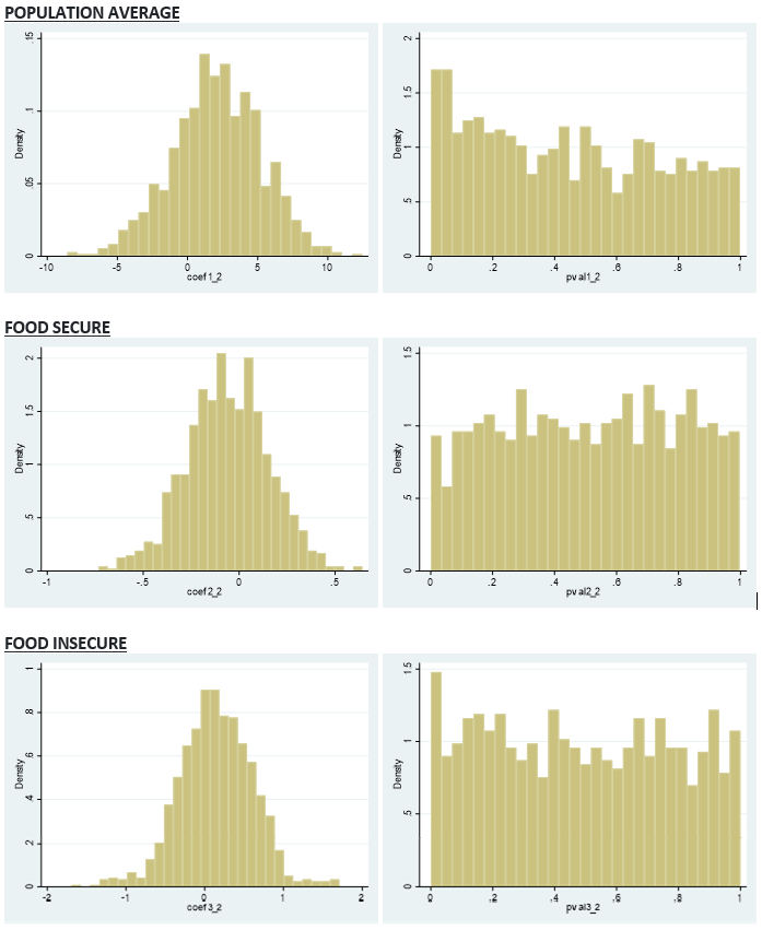
PART 1
Outcome: Fasting glucose level
Exposure: High Education (Less than college vs. College+)
Effect Modifier: Food Insecure
POPULATION AVERAGE
+----------------------------------------------+
| effect_~l pval_all
lower_all upper_all |
|----------------------------------------------|
1. | -14.74748 .0001036
-21.97891 -7.516036 |
2. | -19.41311 1.02e-06
-26.79805 -12.02817 |
3. | -15.66832 6.94e-06
-22.21318 -9.123456 |
4. | -16.7047
.0000105 -23.83653 -9.572883 |
5. | -16.97265 .0000101
-24.20436 -9.740929 |
6. | -16.93757 .0000579
-24.93193 -8.943209 |
7. | -19.65183 4.94e-08
-26.24896 -13.05469 |
8. | -13.21931 .0011712
-21.06437 -5.374257 |
9. | -17.73146 .0000127
-25.38162 -10.0813 |
10.| -21.8019
3.25e-15 -26.43337 -17.17042 |
+----------------------------------------------+
FOOD SECURE
+----------------------------------------------+
| effect_~0 pval_fd0
lower_fd0 upper_fd0 |
|----------------------------------------------|
1. | -19.97094 0
-20.32219 -19.61969 |
2. | -20.29086 0
-20.70551 -19.87621 |
3. | -20.22832 0
-20.65046 -19.80618 |
4. | -20.15899 0
-20.58412 -19.73386 |
5. | -20.04579 0
-20.52253 -19.56904 |
6. | -19.86287 0
-20.25656 -19.46917 |
7. | -20.05218 0
-20.46613 -19.63823 |
8. | -19.86929 0
-20.31412 -19.42447 |
9. | -19.80927 0
-20.27908 -19.33946 |
10.| -20.28098 0
-20.65875 -19.90321 |
+----------------------------------------------+
FOOD INSECURE
+----------------------------------------------+
| effect_~1 pval_fd1
lower_fd1 upper_fd1 |
|----------------------------------------------|
1. | -9.919834 1.38e-09
-11.45002 -8.389648 |
2. | -10.01557 2.78e-11
-11.33897 -8.692163 |
3. | -9.52847
7.44e-10 -10.8339 -8.223036 |
4. | -9.228227 3.30e-11
-10.30346 -8.152988 |
5. | -10.4451
7.79e-13 -11.53759 -9.352617 |
6. | -10.58829 1.28e-18
-11.33111 -9.845469 |
7. | -10.04851 2.08e-10
-11.18128 -8.915744 |
8. | -8.973975 1.17e-13
-9.927564 -8.020388 |
9. | -9.170382 1.03e-13
-10.07702 -8.263741 |
10.| -10.73896 .0000524
-12.90067 -8.577255 |
+----------------------------------------------+
PART 3
Power 1: 0.0785
Power 2: 0.0570
Power 3: From Stata "the control-group mean and the experimental-group mean are equal; this is not allowed"
All above power calculations were computed using the "power" command in Stata. I would appreciate further explanation about the third power calculation (is the point that if there is no difference between the means of two groups, that there is no way to detect a difference?).
Hi Alice,
Do you mind sharing your code with me for drawing the 1000 samples and storing them in STATA? I did a code for the 1000 samples and I stored it in scalars but I have no idea how to generate an histogram with scalars, maybe I should have used another macro?
Thanks!
Monica
Sure thing, Monica! I've attached my do file.
Disclosure: this code was written in collaboration with my classmates. I definitely didn't figure it out myself :)
Thanks, Alice!
Alice
Nice results - can you post your code?
If you think of power is the probability of rejecting the null under the alternative hypothesis, when the alternative is that the two means are the same, power=alpha.
Usually we think of power as the probability of rejecting the null when it is false assuming the null is that m0=m1 (which is why stata is not happy w/ the power calc when you make m0=m1 the alternative hypothesis, the same as the null) but sometimes you need to ask questions about power when the null hypothesis is something besides no difference in means. Suppose for example, that your null hypothesis is that the mean in group 1 is at least 3 points higher than the mean in group 2, and the alternative is that the mean in group 1 is less than 3 points higher than the mean in group 2. You might want to calculate the power to reject the null of a 3+ point difference with any given data set.
Maria
skipping
Exposure: sarcoidosis (yes/no)
Outcome: pulmonary fibrosis (yes/no)
Effect modifier: Black race (yes/no)
In cross sectional analysis the OR for pulmonary fibrosis in Blacks with sarcoidosis was 6.4 times the odds of Whites with sarcoidosis in my US cohort data set
***my only experience with simulations was a handful of times this past year. I tried learning more by reading blogs and videos but after 3 hours, I still don’t know how to generate variables for logistic regression. But I can simulate simple linear regression now such as y = 2 + 3*x + e. Seems like a lot of time to spend without learning a whole lot!! In the end, I had two main problems:
I think I was trying too many complicated formulas for exposure and outcomes such as
gen Pexposure = exp(`g0' + `g1'*U )/(1 + exp(`g0' + `g1'*U)) and trying to specify the ln terms for g0 and g1and I couldn’t get anything to work. And second, I don’t understand my model because I don’t know what the intercept would be (?? 0??) So maybe my model doesn’t make sense. For what it’s worth, I went back to your lecture from Friday and saw the simple simulation you did with SBP which made sense but then I did not know how to mimic that for a binary exposure and outcome. So in the end, this is as far as I could take it
Y= b0 = 0 if no sarcoidosis
Y = b0 + b1*exposure + b2*modifier
PF=0 + b1*sarcoidosis + b2*Black
If you have more examples of simulations that model
linear vs logistic vs count data, etc, I would love to study them.
Laura
Yes- I find it a bit easier to simulate continuous outcomes - for binary this is where the log odds idea is useful because you can generate the log odds as a continuous outcome, and then convert the log odds to an odds (by exponentiating) and the odds to a probability (by using prob=odds/(1+odds)).
As far as choosing an intercept- you can just try some values to see what delivers plausible values. For continuous outcomes, a mean value (eg 25 for BMI) is a good starting point. For binary outcomes, it depends how you are generating the variable but if you use the rule I gave you above, a log odds of -3 delivers a probability of about 5%. A log odds of -2 gives a probability of about 12%.
Maria